2024. 3. 12. 00:26ㆍMOOC
인코딩의 예: 이미지 데이터
from sklearn.datasets import load_digits
import seaborn as sns
import matplotlib.pyplot as plt
import matplotlib as mpl

digits = load_digits()
sns.heatmap(digits.images[0], cmap=mpl.cm.bone_r, annot=True, fmt="2.0f",
            cbar=True, xticklabels=False, yticklabels=False)
plt.title("MNIST 숫자 이미지 표본")
plt.show()
인코딩의 다른 예 : 문서 데이터
from sklearn.datasets import fetch_20newsgroups

news = fetch_20newsgroups()
print("입력:\n", news.data[0])
print("출력:\n", news.target_names[news.target[0]])
입력:
From: lerxst@wam.umd.edu (where's my thing)
Subject: WHAT car is this!?
Nntp-Posting-Host: rac3.wam.umd.edu
Organization: University of Maryland, College Park
Lines: 15
I was wondering if anyone out there could enlighten me on this car I saw
the other day. It was a 2-door sports car, looked to be from the late 60s/
early 70s. It was called a Bricklin. The doors were really small. In addition,
the front bumper was separate from the rest of the body. This is
all I know. If anyone can tellme a model name, engine specs, years
of production, where this car is made, history, or whatever info you
have on this funky looking car, please e-mail.
Thanks,
- IL
---- brought to you by your neighborhood Lerxst ----
출력:
rec.autosfrom sklearn.feature_extraction.text import CountVectorizer
vec = CountVectorizer(stop_words="english").fit(news.data[:100])
data = vec.transform(news.data[:100])
data.shape(100, 6288)sns.heatmap(data.toarray()[:50, :100], cmap=mpl.cm.bone_r,
linewidths=0.001, linecolor='gray', cbar=False,
xticklabels=False, yticklabels=False)
plt.xlabel("단어")
plt.ylabel("문서")
plt.title("BOW(Bag of Words) 인코딩 결과 시각화")
plt.show()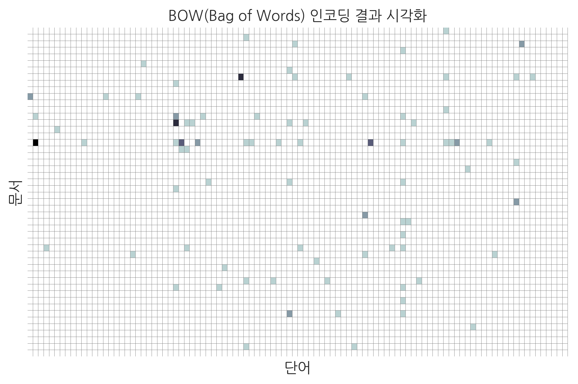
회귀분석의 예
다음은 회귀분석의 한 예로 scikit-learn 패키지에서 제공하는 주택가격을 예측하는 문제를 보였다. 이 문제는 범죄율, 공기 오염도 등의 주거 환경 정보 등을 사용하여 70년대 미국 보스턴시의 주택가격을 예측하는 문제이다.
보스턴 주택가격 데이터
from sklearn.datasets import load_boston

boston = load_boston()
df = pd.DataFrame(boston.data, columns=boston.feature_names)
df["주택가격"] = boston.target
g = sns.pairplot(df[["주택가격", "RM", "AGE", "CRIM"]])
g.fig.suptitle("보스턴 주택가격 데이터 일부 (RM: 방 개수, AGE: 노후화, CRIM: 범죄율)", y=1.02)
plt.show()
이 문제를 회귀분석 방법으로 풀면 다음 결과 그래프와 같다. 결과 그래프에서 하나의 점은 하나의 데이터를 뜻한다. 점의 가로축 값은 실제 가격을 나타내고 세로축 값은 회귀분석 결과이다. 만약 회귀분석 방법으로 가격을 정확하게 예측했다면 결과는 기울기가 1인 직선과 같은 형태가 되어야 하지만 실제로는 타원 모양이 되는 경우가 많다.
보스턴 주택가격 예측결과
from sklearn.linear_model import LinearRegression

model = LinearRegression().fit(boston.data, boston.target)
predicted = model.predict(boston.data)
plt.scatter(boston.target, predicted)
plt.xlabel("실제 가격")
plt.ylabel("예측 가격")
plt.title("보스턴 주택가격 예측결과")
plt.show()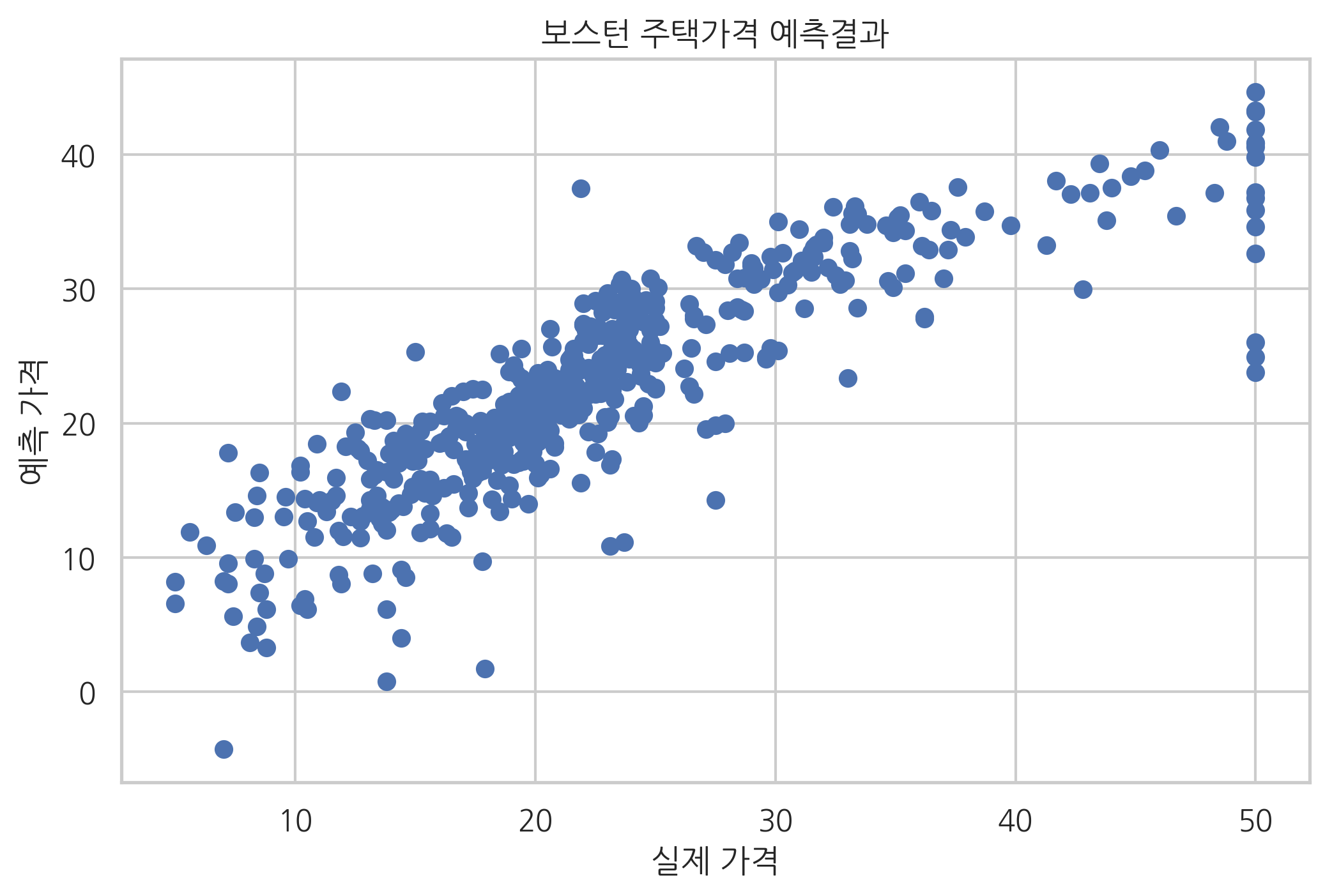
분류의 예
다음은 분류의 한 예로 scikit-learn 패키지에서 제공하는 붓꽃(iris) 분류 문제를 보였다. 이 문제는 붓꽃의 꽃받침 길이(sepal length), 꽃받침 폭(sepal width), 꽃잎 길이(petal length), 꽃잎 폭(petal width)을 이용하여 붓꽃의 세가지 종류(setosa, versicolor, virginica) 중 어느 것에 속하는지를 결정하는 문제이다.
아래에는 파이썬을 이용하여 붓꽃 데이터의 일부와 이를 시각화한 모습을 보였다.
붓꽃 분류 데이터
from sklearn.datasets import load_iris

iris = load_iris()
df = pd.DataFrame(iris.data, columns=iris.feature_names)
sy = pd.Series(iris.target, dtype="category")
sy = sy.cat.rename_categories(iris.target_names)
df['species'] = sy

np.random.seed(0)
df.sample(frac=1).reset_index(drop=True).head(10)
sepal length (cm)sepal width (cm)petal length (cm)petal width (cm)species0123456789
| 5.8 | 2.8 | 5.1 | 2.4 | virginica |
| 6.0 | 2.2 | 4.0 | 1.0 | versicolor |
| 5.5 | 4.2 | 1.4 | 0.2 | setosa |
| 7.3 | 2.9 | 6.3 | 1.8 | virginica |
| 5.0 | 3.4 | 1.5 | 0.2 | setosa |
| 6.3 | 3.3 | 6.0 | 2.5 | virginica |
| 5.0 | 3.5 | 1.3 | 0.3 | setosa |
| 6.7 | 3.1 | 4.7 | 1.5 | versicolor |
| 6.8 | 2.8 | 4.8 | 1.4 | versicolor |
| 6.1 | 2.8 | 4.0 | 1.3 | versicolor |
sns.pairplot(df, hue="species", markers=["o", "s", "x"])
plt.suptitle("붓꽃 데이터", y=1.02, fontsize=18)
plt.show()
from sklearn.preprocessing import StandardScaler
from sklearn.svm import SVC

features = [2, 3]
X = iris.data[:, features]
y = iris.target

model = SVC(kernel="linear", random_state=0)
model.fit(X, y)

XX_min = X[:, 0].min() - 1
XX_max = X[:, 0].max() + 1
YY_min = X[:, 1].min() - 1
YY_max = X[:, 1].max() + 1
XX, YY = np.meshgrid(np.linspace(XX_min, XX_max, 1000),
                     np.linspace(YY_min, YY_max, 1000))
ZZ = model.predict(np.c_[XX.ravel(), YY.ravel()]).reshape(XX.shape)

cmap = mpl.colors.ListedColormap(['seashell', 'lightgreen', 'lightskyblue'])
plt.contourf(XX, YY, ZZ, cmap=cmap)
plt.contour(XX, YY, ZZ, colors='k')
plt.scatter(X[y == 0, 0], X[y == 0, 1], s=20, label=iris.target_names[0],
            marker="o", edgecolors="darkred", facecolors="red")
plt.scatter(X[y == 1, 0], X[y == 1, 1], s=20, label=iris.target_names[1],
            marker="s", edgecolors="darkgreen", facecolors="green")
plt.scatter(X[y == 2, 0], X[y == 2, 1], s=30, label=iris.target_names[2],
            marker="x", edgecolors="darkblue", facecolors="blue")
plt.xlim(XX_min, XX_max)
plt.ylim(YY_min, YY_max)
plt.xlabel("꽃잎의 길이(cm)")
plt.ylabel("꽃잎의 폭(cm)")
plt.title("서포트벡터머신을 이용한 붓꽃 분류 결과")
plt.legend(loc="lower right", framealpha=1)
plt.show()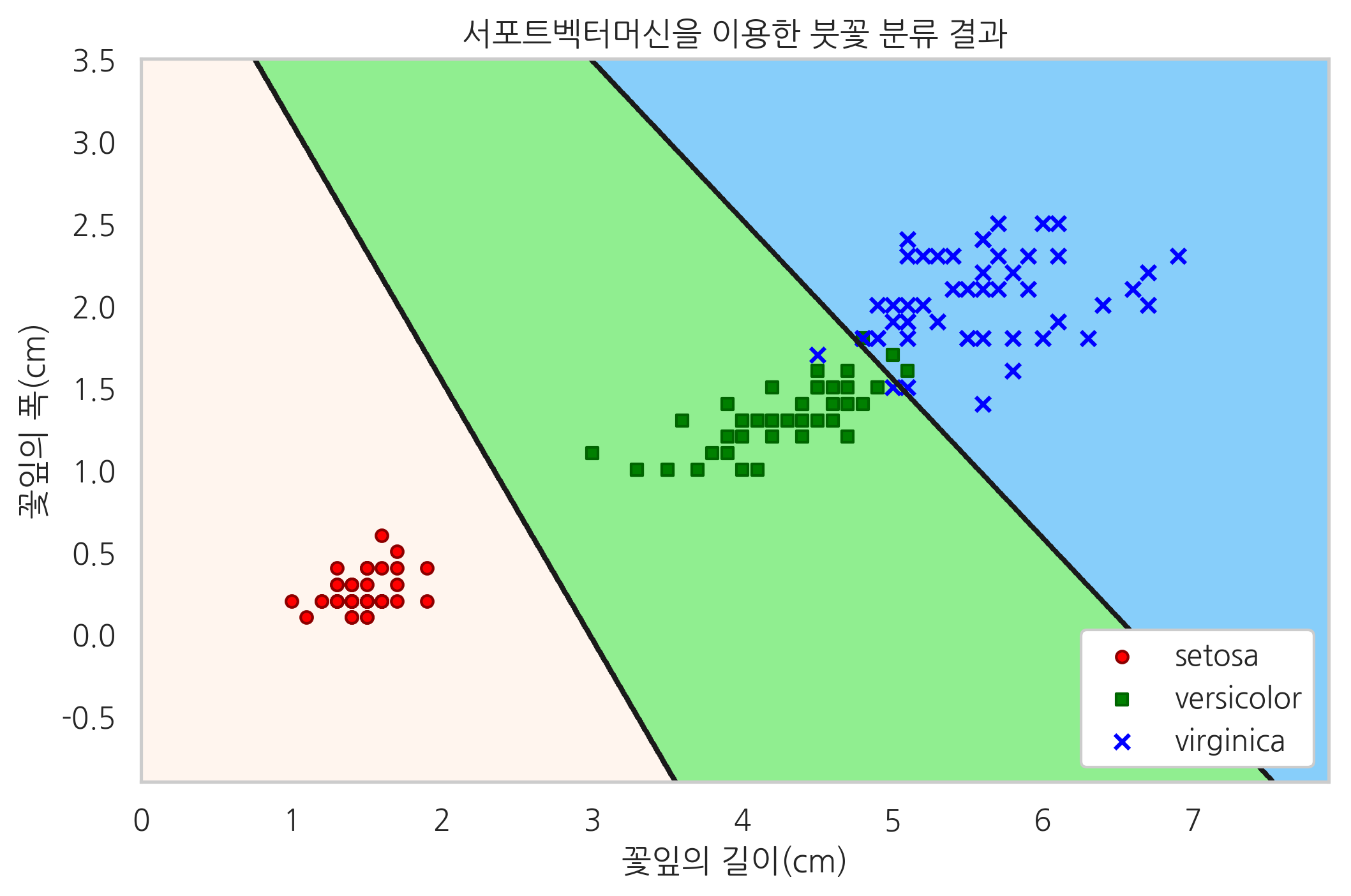
비지도학습
지금까지 살펴본 지도학습에서는 입력값과 출력값의 쌍(pair)을 학습데이터로 하여 입력값에 대한 출력값을 예측하도록 학습을 시켰다. 하지만 때로는 데이터간에 입력과 출력의 관계가 명확하지 않을 수도 있다. 이렇게 입력/출력이 구분되지 않는 단순한 “데이터들의 관계”에서 특정한 규칙을 찾아내는 것을 **비지도학습(unsupervised learning)**이라고 한다. 비지도학습에서는 입력/출력 데이터를 구분짓지 않고 단순히 데이터를 입력하면 이 데이터들간의 규칙을 찾아내거나 미리 지정한 규칙(모형)에 맞는 데이터인지를 구분해 낸다.
클러스터링
대표적인 비지도학습 방법 중 하나는 데이터들을 유사한 데이터까지 같은 그룹으로 모으는 클러스터링(clustering) 방법이다. 다음 예제는 100개의 2차원 데이터들을 affinity propagation이라는 방법으로 클러스터링한 결과이다. 왼쪽 그림은 클러스터링을 하기 전의 데이터들을 나타낸 것이고 오른쪽 그림은 클러스터링으로 모아진 데이터를 나타낸 것이다. 전체 데이터를 3개의 그룹으로 분리할 수 있다는 것을 알 수 있다.
클러스터링 예제
from sklearn.datasets import make_blobs
from sklearn.cluster import AffinityPropagation

X, _ = make_blobs(n_features=2, centers=3, random_state=1)
model = AffinityPropagation().fit(X)

plt.subplot(121)
plt.scatter(X[:, 0], X[:, 1], marker='o', s=10, edgecolor="k")
plt.title("클러스터링 전")
plt.subplot(122)
plt.scatter(X[:, 0], X[:, 1], marker='o', s=10, edgecolor="k")
plt.title("클러스터링 후")
for k in range(3):
    cluster_center = X[model.cluster_centers_indices_[k]]
    for x in X[model.labels_ == k]:
        plt.plot([cluster_center[0], x[0]], [cluster_center[1], x[1]], c="k")

plt.suptitle("Affinity Propagation 방법을 사용한 클러스터링 결과", y=1.03)
plt.tight_layout()
plt.show()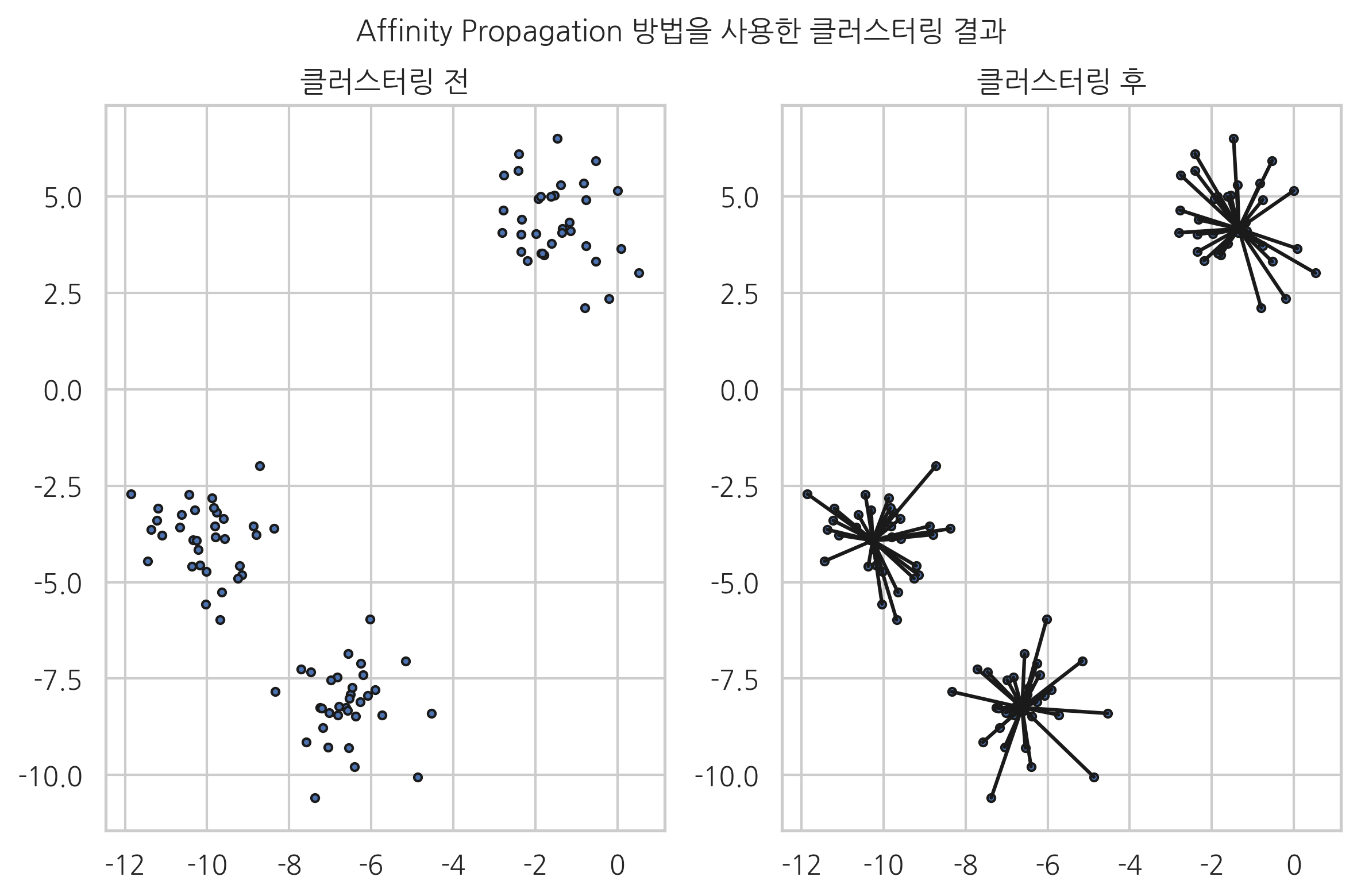
'MOOC' 카테고리의 다른 글
| Scikit-Learn의 문서 전처리 기능 (데이터 사이언스 5) (1) | 2024.03.21 |
|---|---|
| 인공 신경망(Artificial Neural Networks, ANN) 딥러닝 학습1 (0) | 2024.03.14 |
| NLTK 자연어 처리 패키지 (데이터 사이언스 4) (0) | 2024.03.13 |
| 2.1 데이터 전처리 기초 학습 (데이터 사이언스 2) (2) | 2024.03.13 |
| 2.2 범주형 데이터 처리 학습 (데이터 사이언스 3) (3) | 2024.03.12 |