2024. 5. 16. 11:10ㆍ코딩테스트
축구 데이터베이스를 활용하여 리그별 경기당 평균 득점수를 분석해보도록 하겠다. 데이터를 SQLite 데이터베이스에서 가져와 Pandas를 이용해 조작하고, Matplotlib를 통해 시각화할 것이다.
1. 데이터베이스 연결 및 테이블 확인
먼저, SQLite 데이터베이스와 연결하여 테이블 목록을 확인하였다. 이를 통해 데이터베이스에 어떤 테이블이 있는지 파악할 수 있었다.
2. 국가 리스트 확인
Country 테이블을 조회하여 데이터베이스에 저장된 축구 리그가 있는 국가들을 확인하였다. 이를 통해 어떤 국가의 리그들이 데이터베이스에 포함되어 있는지 알 수 있었다.
3. 리그와 국가 테이블 조인
League 테이블과 Country 테이블을 조인하여 각 리그가 어떤 국가에 속해 있는지 정보를 가져왔다. 이 정보를 통해 리그와 국가 간의 관계를 명확히 이해할 수 있었다.
4. 팀 리스트 확인
Team 테이블을 조회하여 데이터베이스에 저장된 팀 목록을 확인하였다. 이는 각 리그에 소속된 팀들을 파악하는 데 도움이 되었다.
5. 스페인 리그 경기 상세 데이터 확인
스페인 리그의 경기 데이터를 조회하여 경기의 세부 정보를 확인하였다. 여기서는 경기 날짜, 홈 팀과 원정 팀, 득점 등의 정보를 포함하였다.
6. 리그별 시즌 평균 득점수 분석
리그별 시즌 평균 득점수를 분석하기 위해 SQL 쿼리를 실행하였다. 분석 대상은 스페인, 독일, 프랑스, 이탈리아, 잉글랜드의 주요 리그였다. 각 시즌 동안 경기당 평균 득점수를 계산하여 리그별 득점 패턴을 비교할 수 있었다.
7. 데이터 프레임 생성 및 시각화
리그별 시즌 평균 득점수를 데이터 프레임으로 생성하고 이를 시각화하였다. 시각화를 통해 리그별로 시즌 동안 경기당 평균 득점수가 어떻게 변화했는지 한눈에 파악할 수 있었다.
#Improts
import numpy as np
import pandas as pd
import sqlite3
import matplotlib.pyplot as plt

database = "C:/Users/82106/Desktop/데이터 분석 프로젝트 2/SQL analyst/data/archive/database.sqlite"  #Insert path here
DB 와 연결후 테이블 확인하기
데이터베이스 연결 및 테이블 확인
우선 SQLite 데이터베이스와 연결하고, 테이블을 확인
conn = sqlite3.connect(database)

tables = pd.read_sql("""SELECT *
                        FROM sqlite_master
                        WHERE type='table';""", conn)
tables
| table | sqlite_sequence | sqlite_sequence | 4 | CREATE TABLE sqlite_sequence(name,seq) |
| table | Player_Attributes | Player_Attributes | 11 | CREATE TABLE "Player_Attributes" (\n\t`id`\tIN... |
| table | Player | Player | 14 | CREATE TABLE `Player` (\n\t`id`\tINTEGER PRIMA... |
| table | Match | Match | 18 | CREATE TABLE `Match` (\n\t`id`\tINTEGER PRIMAR... |
| table | League | League | 24 | CREATE TABLE `League` (\n\t`id`\tINTEGER PRIMA... |
| table | Country | Country | 26 | CREATE TABLE `Country` (\n\t`id`\tINTEGER PRIM... |
| table | Team | Team | 29 | CREATE TABLE "Team" (\n\t`id`\tINTEGER PRIMARY... |
| table | Team_Attributes | Team_Attributes | 2 | CREATE TABLE `Team_Attributes` (\n\t`id`\tINTE... |
국가 리스트 확인
국가 리스트를 확인하기 위해 Country 테이블을 조회한다.
countries=pd.read_sql("""SELECT *
                        FROM Country;""", conn)

countries
| 1 | Belgium |
| 1729 | England |
| 4769 | France |
| 7809 | Germany |
| 10257 | Italy |
| 13274 | Netherlands |
| 15722 | Poland |
| 17642 | Portugal |
| 19694 | Scotland |
| 21518 | Spain |
| 24558 | Switzerland |
테이블 조인하기
League 와 Country 조인
League와 Country 테이블을 조인하여 리그와 국가 정보를 가져온다.
leagues=pd.read_sql("""SELECT*
                    FROM League
                    JOIN Country ON Country.id = League.country_id;""", conn)

leagues
| 1 | 1 | Belgium Jupiler League | 1 | Belgium |
| 1729 | 1729 | England Premier League | 1729 | England |
| 4769 | 4769 | France Ligue 1 | 4769 | France |
| 7809 | 7809 | Germany 1. Bundesliga | 7809 | Germany |
| 10257 | 10257 | Italy Serie A | 10257 | Italy |
| 13274 | 13274 | Netherlands Eredivisie | 13274 | Netherlands |
| 15722 | 15722 | Poland Ekstraklasa | 15722 | Poland |
| 17642 | 17642 | Portugal Liga ZON Sagres | 17642 | Portugal |
| 19694 | 19694 | Scotland Premier League | 19694 | Scotland |
| 21518 | 21518 | Spain LIGA BBVA | 21518 | Spain |
| 24558 | 24558 | Switzerland Super League | 24558 | Switzerland |
팀의 리스트
팀 리스트를 확인하기 위해 Team 테이블을 조회한다
teams=pd.read_sql("""select *
                  from Team
                  order by team_long_name
                  limit 10;""",conn)

teams
| 16848 | 8350 | 29 | 1. FC Kaiserslautern | KAI |
| 15624 | 8722 | 31 | 1. FC Köln | FCK |
| 16239 | 8165 | 171 | 1. FC Nürnberg | NUR |
| 16243 | 9905 | 169 | 1. FSV Mainz 05 | MAI |
| 11817 | 8576 | 614 | AC Ajaccio | AJA |
| 11074 | 108893 | 111989 | AC Arles-Avignon | ARL |
| 49116 | 6493 | 1714 | AC Bellinzona | BEL |
| 26560 | 10217 | 650 | ADO Den Haag | HAA |
| 9537 | 8583 | 57 | AJ Auxerre | AUX |
| 9547 | 9829 | 69 | AS Monaco | MON |
스페인 리그 경기 상세 데이터 확인
스페인 리그의 경기 데이터를 조회한다.
detailed_matches=pd.read_sql("""select Match.id,
                             Country.name as country_name,
                            League.name as league_name,
                            season,
                            stage,
                            date,
                            HT.team_long_name as  home_team,
                            AT.team_long_name as away_team,
                            home_team_goal,
                            away_team_goal
                            from Match
                            join Country on Country.id = Match.country_id
                            join League on League.id = Match.league_id
                            left join Team as HT on HT.team_api_id = Match.home_team_api_id
                            left join Team as AT on AT.team_api_id = Match.away_team_api_id
                            where country_name = 'Spain'
                            order by date
                            limit 10;""",conn)
leages_by_season=pd.read_sql("""SELECT Country.name AS country_name,
                                        League.name AS league_name,
                                        season,
                                        count(distinct stage) AS number_of_stages,
                                        count(distinct HT.team_long_name) AS number_of_teams,
                                        avg(home_team_goal) AS avg_home_team_scors,
                                        avg(away_team_goal) AS avg_away_team_goals,
                                        avg(home_team_goal-away_team_goal) AS avg_goal_dif,
                                        avg(home_team_goal+away_team_goal) AS avg_goals,
                                        sum(home_team_goal+away_team_goal) AS total_goals
                                FROM Match
                                JOIN Country on Country.id = Match.country_id
                                JOIN League on League.id = Match.league_id
                                LEFT JOIN Team AS HT on HT.team_api_id = Match.home_team_api_id
                                LEFT JOIN Team AS AT on AT.team_api_id = Match.away_team_api_id
                                WHERE country_name in ('Spain', 'Germany', 'France', 'Italy', 'England')
                                GROUP BY Country.name, League.name, season
                                HAVING count(distinct stage) > 10
                                ORDER BY Country.name, League.name, season DESC
                                ;""", conn)

leages_by_season
| England | England Premier League | 2015/2016 | 38 | 20 | 1.492105 | 1.207895 | 0.284211 | 2.700000 | 1026 |
| England | England Premier League | 2014/2015 | 38 | 20 | 1.473684 | 1.092105 | 0.381579 | 2.565789 | 975 |
| England | England Premier League | 2013/2014 | 38 | 20 | 1.573684 | 1.194737 | 0.378947 | 2.768421 | 1052 |
| England | England Premier League | 2012/2013 | 38 | 20 | 1.557895 | 1.239474 | 0.318421 | 2.797368 | 1063 |
| England | England Premier League | 2011/2012 | 38 | 20 | 1.589474 | 1.215789 | 0.373684 | 2.805263 | 1066 |
| England | England Premier League | 2010/2011 | 38 | 20 | 1.623684 | 1.173684 | 0.450000 | 2.797368 | 1063 |
| England | England Premier League | 2009/2010 | 38 | 20 | 1.697368 | 1.073684 | 0.623684 | 2.771053 | 1053 |
| England | England Premier League | 2008/2009 | 38 | 20 | 1.400000 | 1.078947 | 0.321053 | 2.478947 | 942 |
| France | France Ligue 1 | 2015/2016 | 38 | 20 | 1.436842 | 1.089474 | 0.347368 | 2.526316 | 960 |
| France | France Ligue 1 | 2014/2015 | 38 | 20 | 1.410526 | 1.081579 | 0.328947 | 2.492105 | 947 |
| France | France Ligue 1 | 2013/2014 | 38 | 20 | 1.415789 | 1.039474 | 0.376316 | 2.455263 | 933 |
| France | France Ligue 1 | 2012/2013 | 38 | 20 | 1.468421 | 1.076316 | 0.392105 | 2.544737 | 967 |
| France | France Ligue 1 | 2011/2012 | 38 | 20 | 1.473684 | 1.042105 | 0.431579 | 2.515789 | 956 |
| France | France Ligue 1 | 2010/2011 | 38 | 20 | 1.342105 | 1.000000 | 0.342105 | 2.342105 | 890 |
| France | France Ligue 1 | 2009/2010 | 38 | 20 | 1.389474 | 1.021053 | 0.368421 | 2.410526 | 916 |
| France | France Ligue 1 | 2008/2009 | 38 | 20 | 1.286842 | 0.971053 | 0.315789 | 2.257895 | 858 |
| Germany | Germany 1. Bundesliga | 2015/2016 | 34 | 18 | 1.565359 | 1.264706 | 0.300654 | 2.830065 | 866 |
| Germany | Germany 1. Bundesliga | 2014/2015 | 34 | 18 | 1.588235 | 1.166667 | 0.421569 | 2.754902 | 843 |
| Germany | Germany 1. Bundesliga | 2013/2014 | 34 | 18 | 1.748366 | 1.411765 | 0.336601 | 3.160131 | 967 |
| Germany | Germany 1. Bundesliga | 2012/2013 | 34 | 18 | 1.591503 | 1.343137 | 0.248366 | 2.934641 | 898 |
| Germany | Germany 1. Bundesliga | 2011/2012 | 34 | 18 | 1.660131 | 1.199346 | 0.460784 | 2.859477 | 875 |
| Germany | Germany 1. Bundesliga | 2010/2011 | 34 | 18 | 1.647059 | 1.274510 | 0.372549 | 2.921569 | 894 |
| Germany | Germany 1. Bundesliga | 2009/2010 | 34 | 18 | 1.513072 | 1.316993 | 0.196078 | 2.830065 | 866 |
| Germany | Germany 1. Bundesliga | 2008/2009 | 34 | 18 | 1.699346 | 1.222222 | 0.477124 | 2.921569 | 894 |
| Italy | Italy Serie A | 2015/2016 | 38 | 20 | 1.471053 | 1.105263 | 0.365789 | 2.576316 | 979 |
| Italy | Italy Serie A | 2014/2015 | 38 | 20 | 1.498681 | 1.187335 | 0.311346 | 2.686016 | 1018 |
| Italy | Italy Serie A | 2013/2014 | 38 | 20 | 1.536842 | 1.186842 | 0.350000 | 2.723684 | 1035 |
| Italy | Italy Serie A | 2012/2013 | 38 | 20 | 1.494737 | 1.144737 | 0.350000 | 2.639474 | 1003 |
| Italy | Italy Serie A | 2011/2012 | 38 | 20 | 1.511173 | 1.072626 | 0.438547 | 2.583799 | 925 |
| Italy | Italy Serie A | 2010/2011 | 38 | 20 | 1.431579 | 1.081579 | 0.350000 | 2.513158 | 955 |
| Italy | Italy Serie A | 2009/2010 | 38 | 20 | 1.542105 | 1.068421 | 0.473684 | 2.610526 | 992 |
| Italy | Italy Serie A | 2008/2009 | 38 | 20 | 1.521053 | 1.078947 | 0.442105 | 2.600000 | 988 |
| Spain | Spain LIGA BBVA | 2015/2016 | 38 | 20 | 1.618421 | 1.126316 | 0.492105 | 2.744737 | 1043 |
| Spain | Spain LIGA BBVA | 2014/2015 | 38 | 20 | 1.536842 | 1.118421 | 0.418421 | 2.655263 | 1009 |
| Spain | Spain LIGA BBVA | 2013/2014 | 38 | 20 | 1.631579 | 1.118421 | 0.513158 | 2.750000 | 1045 |
| Spain | Spain LIGA BBVA | 2012/2013 | 38 | 20 | 1.686842 | 1.184211 | 0.502632 | 2.871053 | 1091 |
| Spain | Spain LIGA BBVA | 2011/2012 | 38 | 20 | 1.678947 | 1.084211 | 0.594737 | 2.763158 | 1050 |
| Spain | Spain LIGA BBVA | 2010/2011 | 38 | 20 | 1.636842 | 1.105263 | 0.531579 | 2.742105 | 1042 |
| Spain | Spain LIGA BBVA | 2009/2010 | 38 | 20 | 1.600000 | 1.113158 | 0.486842 | 2.713158 | 1031 |
| Spain | Spain LIGA BBVA | 2008/2009 | 38 | 20 | 1.660526 | 1.236842 | 0.423684 | 2.897368 | 1101 |
df= pd.DataFrame (index=np.sort(leages_by_season['season'].unique()), columns= leages_by_season['country_name'].unique())

df.loc[:,'Germany']= list(leages_by_season.loc[leages_by_season['country_name']=='Germany','avg_goals'])
df.loc[:,'Spain']=list(leages_by_season.loc[leages_by_season['country_name']=='Spain','avg_goals'])
df.loc[:,'France']   = list(leages_by_season.loc[leages_by_season['country_name']=='France','avg_goals'])
df.loc[:,'Italy']   = list(leages_by_season.loc[leages_by_season['country_name']=='Italy','avg_goals'])
df.loc[:,'England']   = list(leages_by_season.loc[leages_by_season['country_name']=='England','avg_goals'])

df.plot(figsize=(12,5),title='Average Goals per Game Over Time')
<Axes: title={'center': 'Average Goals per Game Over Time'}>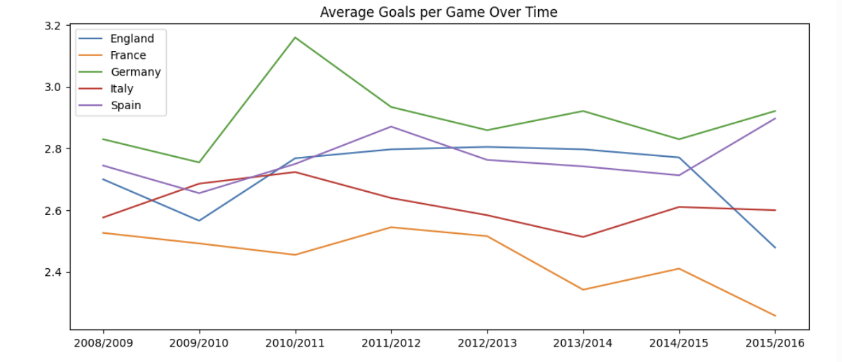
df = pd.DataFrame(index=np.sort(leages_by_season['season'].unique()), columns=leages_by_season['country_name'].unique())

df.loc[:,'Germany'] = list(leages_by_season.loc[leages_by_season['country_name']=='Germany','avg_goal_dif'])
df.loc[:,'Spain']   = list(leages_by_season.loc[leages_by_season['country_name']=='Spain','avg_goal_dif'])
df.loc[:,'France']   = list(leages_by_season.loc[leages_by_season['country_name']=='France','avg_goal_dif'])
df.loc[:,'Italy']   = list(leages_by_season.loc[leages_by_season['country_name']=='Italy','avg_goal_dif'])
df.loc[:,'England']   = list(leages_by_season.loc[leages_by_season['country_name']=='England','avg_goal_dif'])

df.plot(figsize=(12,5),title='Average Goals Difference Home vs Out')
players_height = pd.read_sql("""SELECT CASE
                                        WHEN ROUND(height)<165 then 165
                                        WHEN ROUND(height)>195 then 195
                                        ELSE ROUND(height)
                                        END AS calc_height,
                                        COUNT(height) AS distribution,
                                        (avg(PA_Grouped.avg_overall_rating)) AS avg_overall_rating,
                                        (avg(PA_Grouped.avg_potential)) AS avg_potential,
                                        AVG(weight) AS avg_weight
                            FROM PLAYER
                            LEFT JOIN (SELECT Player_Attributes.player_api_id,
                                        avg(Player_Attributes.overall_rating) AS avg_overall_rating,
                                        avg(Player_Attributes.potential) AS avg_potential
                                        FROM Player_Attributes
                                        GROUP BY Player_Attributes.player_api_id)
                                        AS PA_Grouped ON PLAYER.player_api_id = PA_Grouped.player_api_id
                            GROUP BY calc_height
                            ORDER BY calc_height
                                ;""", conn)
players_height
| 165.0 | 74 | 67.365543 | 73.327754 | 139.459459 |
| 168.0 | 118 | 67.500518 | 73.124182 | 144.127119 |
| 170.0 | 403 | 67.726903 | 73.379056 | 147.799007 |
| 173.0 | 530 | 66.980272 | 72.848746 | 152.824528 |
| 175.0 | 1188 | 66.805204 | 72.258774 | 156.111953 |
| 178.0 | 1489 | 66.367212 | 71.943339 | 160.665547 |
| 180.0 | 1388 | 66.419053 | 71.846394 | 165.261527 |
| 183.0 | 1954 | 66.634380 | 71.754555 | 170.167861 |
| 185.0 | 1278 | 66.928964 | 71.833475 | 174.636933 |
| 188.0 | 1305 | 67.094253 | 72.151949 | 179.278161 |
| 191.0 | 652 | 66.997649 | 71.846159 | 184.791411 |
| 193.0 | 470 | 67.485141 | 72.459225 | 188.795745 |
| 195.0 | 211 | 67.425619 | 72.615373 | 196.464455 |
# calc_height 열을 정수형으로 변환
players_height['calc_height'] = players_height['calc_height'].astype(int)
# 그래프 그리기
players_height.plot(x='calc_height', y='avg_overall_rating', figsize=(12, 5), title='Potential vs Height')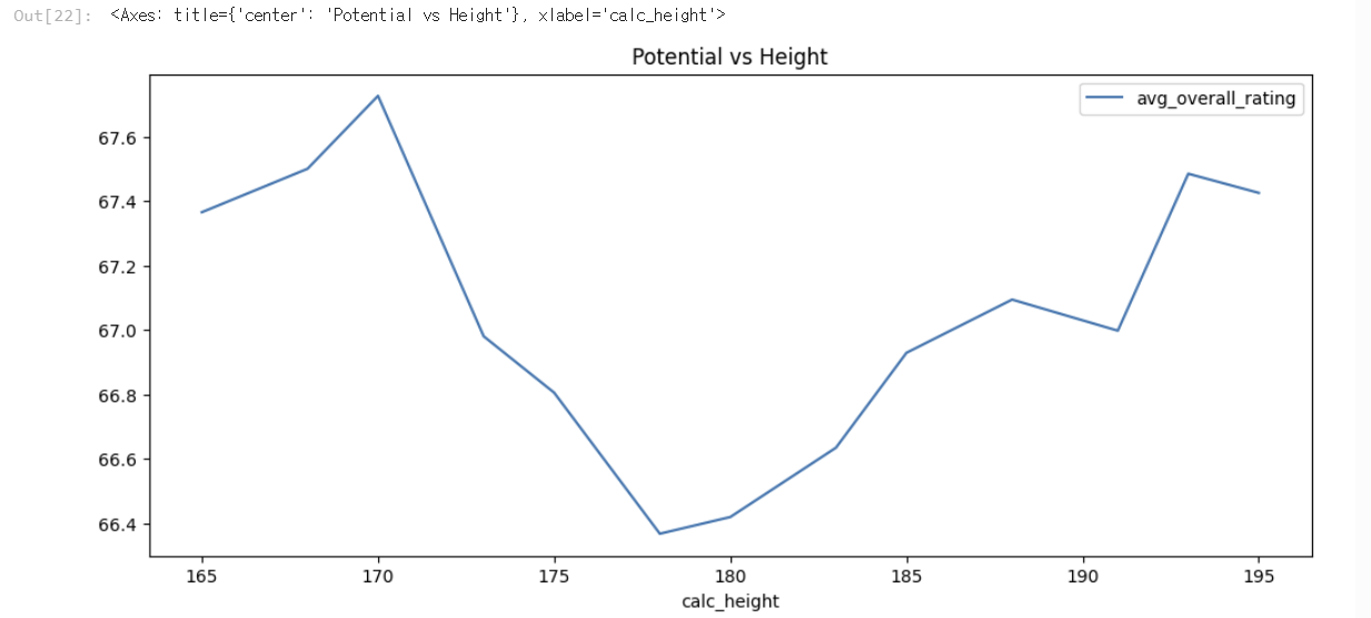
# 선수들의 평균 나이와 포지션별 데이터 분석 수정
players_position_age = pd.read_sql("""
    SELECT position,
           ROUND(AVG(age), 2) AS avg_age,
           COUNT(*) AS player_count
    FROM (
        SELECT P.player_api_id,
               CASE
                   WHEN (AVG(PA.overall_rating) + AVG(PA.potential)) / 2 >= 75 THEN 'Top Player'
                   ELSE 'Regular Player'
               END AS position,
               (julianday('now') - julianday(P.birthday)) / 365 AS age
        FROM Player AS P
        LEFT JOIN Player_Attributes AS PA ON P.player_api_id = PA.player_api_id
        GROUP BY P.player_api_id
    )
    GROUP BY position
    ORDER BY avg_age;
""", conn)

players_position_age
| Regular Player | 37.00 | 9228 |
| Top Player | 38.84 | 1832 |
리그별 시즌 평균 득점수 분석
리그별 시즌 평균 득점수를 분석하기 위해 SQL 쿼리를 실행한다.
# 리그별 시즌 평균 득점수 분석

league_season_goals=pd.read_sql("""select Country.name as country_name,
                                League.name as league_name,
                                season,
                                avg(home_team_goal+away_team_goal) as avg_goals
                                from Match
                                join Country on Country.id=Match.country_id
                                join League on League.id=Match.league_id
                                where country_name in ('Spain', 'Germany', 'France', 'Italy', 'England')
                                group by Country.name,League.name,season
                                order by country.name, League.name,season;""",conn)

league_season_goals
| England | England Premier League | 2008/2009 | 2.478947 |
| England | England Premier League | 2009/2010 | 2.771053 |
| England | England Premier League | 2010/2011 | 2.797368 |
| England | England Premier League | 2011/2012 | 2.805263 |
| England | England Premier League | 2012/2013 | 2.797368 |
| England | England Premier League | 2013/2014 | 2.768421 |
| England | England Premier League | 2014/2015 | 2.565789 |
| England | England Premier League | 2015/2016 | 2.700000 |
| France | France Ligue 1 | 2008/2009 | 2.257895 |
| France | France Ligue 1 | 2009/2010 | 2.410526 |
| France | France Ligue 1 | 2010/2011 | 2.342105 |
| France | France Ligue 1 | 2011/2012 | 2.515789 |
| France | France Ligue 1 | 2012/2013 | 2.544737 |
| France | France Ligue 1 | 2013/2014 | 2.455263 |
| France | France Ligue 1 | 2014/2015 | 2.492105 |
| France | France Ligue 1 | 2015/2016 | 2.526316 |
| Germany | Germany 1. Bundesliga | 2008/2009 | 2.921569 |
| Germany | Germany 1. Bundesliga | 2009/2010 | 2.830065 |
| Germany | Germany 1. Bundesliga | 2010/2011 | 2.921569 |
| Germany | Germany 1. Bundesliga | 2011/2012 | 2.859477 |
| Germany | Germany 1. Bundesliga | 2012/2013 | 2.934641 |
| Germany | Germany 1. Bundesliga | 2013/2014 | 3.160131 |
| Germany | Germany 1. Bundesliga | 2014/2015 | 2.754902 |
| Germany | Germany 1. Bundesliga | 2015/2016 | 2.830065 |
| Italy | Italy Serie A | 2008/2009 | 2.600000 |
| Italy | Italy Serie A | 2009/2010 | 2.610526 |
| Italy | Italy Serie A | 2010/2011 | 2.513158 |
| Italy | Italy Serie A | 2011/2012 | 2.583799 |
| Italy | Italy Serie A | 2012/2013 | 2.639474 |
| Italy | Italy Serie A | 2013/2014 | 2.723684 |
| Italy | Italy Serie A | 2014/2015 | 2.686016 |
| Italy | Italy Serie A | 2015/2016 | 2.576316 |
| Spain | Spain LIGA BBVA | 2008/2009 | 2.897368 |
| Spain | Spain LIGA BBVA | 2009/2010 | 2.713158 |
| Spain | Spain LIGA BBVA | 2010/2011 | 2.742105 |
| Spain | Spain LIGA BBVA | 2011/2012 | 2.763158 |
| Spain | Spain LIGA BBVA | 2012/2013 | 2.871053 |
| Spain | Spain LIGA BBVA | 2013/2014 | 2.750000 |
| Spain | Spain LIGA BBVA | 2014/2015 | 2.655263 |
| Spain | Spain LIGA BBVA | 2015/2016 | 2.744737 |
# 데이터 프레임 생성
df_league_season = pd.DataFrame(index=np.sort(league_season_goals['season'].unique()), columns=league_season_goals['country_name'].unique())

# 각 리그별로 평균 득점 수를 데이터 프레임에 추가
for country in league_season_goals['country_name'].unique():
    df_league_season.loc[:, country] = list(league_season_goals.loc[league_season_goals['country_name'] == country, 'avg_goals'])

# 시각화
df_league_season.plot(figsize=(12, 5), title='Average Goals per Game Over Time by League')
plt.show()
결론
이 분석을 통해 각 리그별로 시즌 동안 경기당 평균 득점수가 어떻게 변화했는지 시각적으로 확인할 수 있었다. 이러한 분석은 축구 경기의 득점 패턴을 이해하는 데 도움을 줄 수 있으며, 리그 간의 차이를 비교하는 데 유용하다.
'코딩테스트' 카테고리의 다른 글
| 프로그래머스 SQL LEVEL4 "우유와 요거트가 담긴 장바구니" (0) | 2025.07.19 |
|---|---|
| [Python] Python 코딩테스트 Level 1 (0) | 2024.05.19 |
| [SQL] 프로그래머스 7 Level 2 (4) | 2024.05.02 |
| [SQL] SQL과 python 연동을 통하여 aircrafts_data 분석 (0) | 2024.05.02 |
| [SQL] 프로그래머스 6 (1) | 2024.04.11 |