2024. 12. 20. 02:15ㆍMOOC
Deeper Layers의 문제
Convolution을 더 깊게 쌓기
AlexNet과 VGGNet이 등장하면서 네트워크가 깊어질수록 receptive field가 커지고 복잡한 관계를 학습할 수 있다는 특징이 확인되었다. 하지만 네트워크를 단순히 깊게 쌓는다고 해서 성능이 무조건 향상되는 것은 아니었다.
최적화의 어려움
깊은 네트워크는 Gradient Vanishing/Exploding 문제로 인해 최적화가 어려워지는 문제가 있었다. 이로 인해 계산 복잡도가 증가하고 하드웨어 요구사항이 까다로워지는 등의 문제가 발생한다.
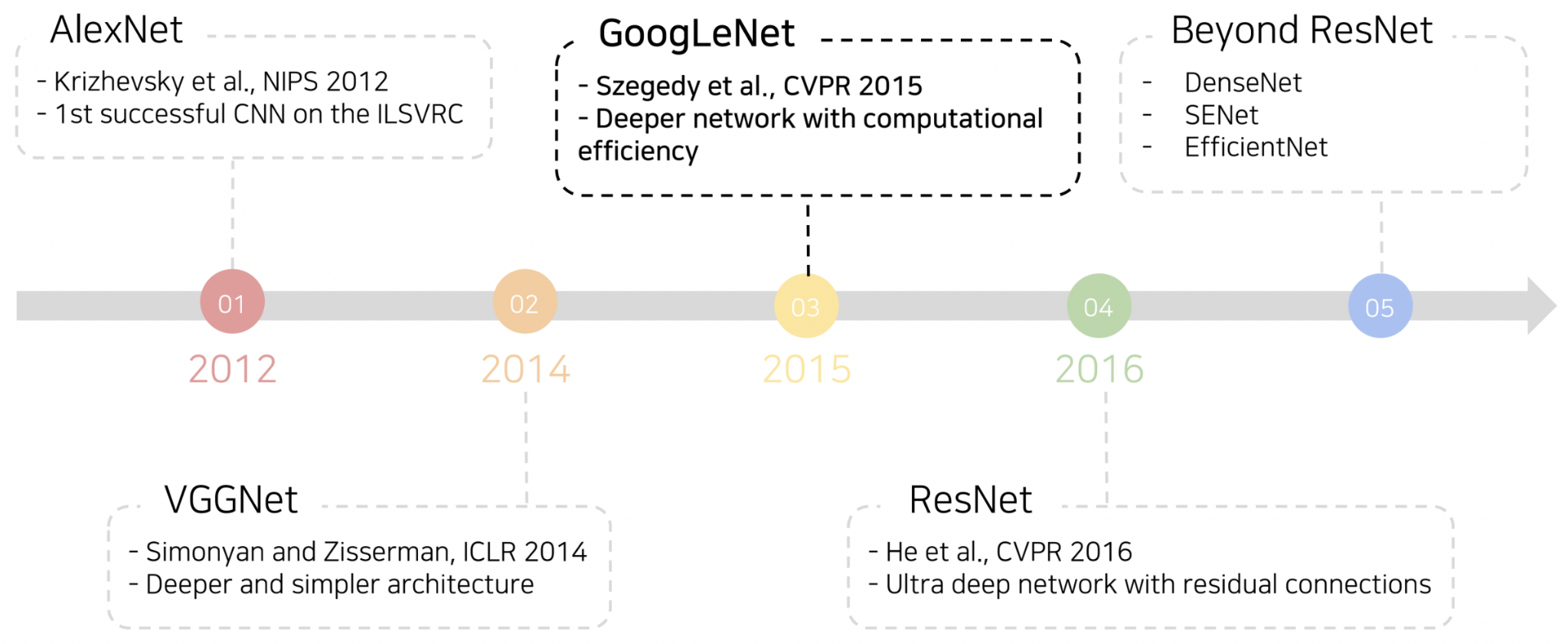
CNN 기반 이미지 분류 아키텍처의 발전
GoogLeNet
GoogLeNet은 Inception module이라는 새로운 구조를 제안한 네트워크이다. Inception module은 하나의 층에서 다양한 크기의 필터를 활용하고, 각 필터를 거친 출력 값을 channel 축으로 concat하여 다양한 특징을 추출하는 방식이다.

많은 필터를 사용할 경우 파라미터와 계산량이 증가하게 되므로, 1x1 convolution 필터를 사용하여 channel dimension을 줄이는 방식을 도입하였다.

GoogLeNet의 전체 구조는 vanilla convolution network로 구성된 Stem network, 중첩된 Inception module, 그리고 auxiliary classifier로 이루어져 있다. Auxiliary classifier는 gradient vanishing 문제를 완화하기 위해 네트워크 중간에 추가로 gradient를 주입하는 역할을 한다. 이는 학습 과정에서만 사용되고 테스트 시에는 사용되지 않는다.

import tensorflow as tf
from tensorflow.keras.layers import Conv2D, MaxPooling2D, AveragePooling2D, Flatten, Dense, Input, Dropout, concatenate
from tensorflow.keras.models import Model

# Inception Module 정의
def inception_module(x, f1, f3_in, f3, f5_in, f5, pool_proj):
    # 1x1 Conv
    conv1 = Conv2D(f1, (1, 1), padding='same', activation='relu')(x)

    # 1x1 Conv -> 3x3 Conv
    conv3 = Conv2D(f3_in, (1, 1), padding='same', activation='relu')(x)
    conv3 = Conv2D(f3, (3, 3), padding='same', activation='relu')(conv3)

    # 1x1 Conv -> 5x5 Conv
    conv5 = Conv2D(f5_in, (1, 1), padding='same', activation='relu')(x)
    conv5 = Conv2D(f5, (5, 5), padding='same', activation='relu')(conv5)

    # MaxPooling -> 1x1 Conv
    pool = MaxPooling2D((3, 3), strides=(1, 1), padding='same')(x)
    pool = Conv2D(pool_proj, (1, 1), padding='same', activation='relu')(pool)

    # Concat 모든 branch
    output = concatenate([conv1, conv3, conv5, pool], axis=-1)
    return output

# Auxiliary Classifier 정의
def auxiliary_classifier(x, num_classes):
    x = AveragePooling2D((5, 5), strides=(3, 3))(x)
    x = Conv2D(128, (1, 1), padding='same', activation='relu')(x)
    x = Flatten()(x)
    x = Dense(1024, activation='relu')(x)
    x = Dropout(0.7)(x)
    x = Dense(num_classes, activation='softmax')(x)
    return x

# GoogLeNet 모델 정의
def googlenet(input_shape=(224, 224, 3), num_classes=1000):
    inputs = Input(shape=input_shape)

    # Stem Network
    x = Conv2D(64, (7, 7), strides=(2, 2), padding='same', activation='relu')(inputs)
    x = MaxPooling2D((3, 3), strides=(2, 2), padding='same')(x)
    x = Conv2D(64, (1, 1), padding='same', activation='relu')(x)
    x = Conv2D(192, (3, 3), padding='same', activation='relu')(x)
    x = MaxPooling2D((3, 3), strides=(2, 2), padding='same')(x)

    # Inception Modules
    x = inception_module(x, 64, 96, 128, 16, 32, 32)
    x = inception_module(x, 128, 128, 192, 32, 96, 64)
    x = MaxPooling2D((3, 3), strides=(2, 2), padding='same')(x)

    x = inception_module(x, 192, 96, 208, 16, 48, 64)
    aux1 = auxiliary_classifier(x, num_classes)  # Auxiliary Classifier 1

    x = inception_module(x, 160, 112, 224, 24, 64, 64)
    x = inception_module(x, 128, 128, 256, 24, 64, 64)
    x = inception_module(x, 112, 144, 288, 32, 64, 64)
    aux2 = auxiliary_classifier(x, num_classes)  # Auxiliary Classifier 2

    x = inception_module(x, 256, 160, 320, 32, 128, 128)
    x = MaxPooling2D((3, 3), strides=(2, 2), padding='same')(x)

    x = inception_module(x, 256, 160, 320, 32, 128, 128)
    x = inception_module(x, 384, 192, 384, 48, 128, 128)

    # Final Output
    x = AveragePooling2D((7, 7), strides=(1, 1))(x)
    x = Flatten()(x)
    x = Dropout(0.4)(x)
    outputs = Dense(num_classes, activation='softmax')(x)

    # 모델 정의 (Auxiliary Classifier 포함)
    model = Model(inputs, [outputs, aux1, aux2])
    return model

# GoogLeNet 모델 생성
model = googlenet(input_shape=(224, 224, 3), num_classes=10)
model.summary()
ResNet
ResNet은 100개 이상의 깊은 층을 가지면서 ImageNet에서 인간보다 뛰어난 성능을 처음으로 달성한 네트워크이다. 깊은 층을 쌓을수록 성능이 좋아질 수 있음을 보여준 첫 사례이다. 하지만 이전 연구에서 층이 깊어질수록 발생하는 문제들 때문에 실패했던 사례들도 많았다.
ResNet은 이러한 문제를 해결하기 위해 shortcut connection(또는 residual connection)을 제안하였다. 일반적으로 입력값 x에서 직접 H(x)를 학습하기보다는, 입력값에서 identity x를 제외한 나머지 F(x)만을 모델링하여 학습하는 방식으로 학습 부담을 줄였다.

Residual block의 수를 n이라 할 때, gradient는 2^n개의 다른 경로로 흐를 수 있게 설계되었다. 이렇게 다양한 경로를 통해 복잡한 매핑을 학습할 수 있었고, 이로 인해 성능이 향상되었다고 할 수 있다.
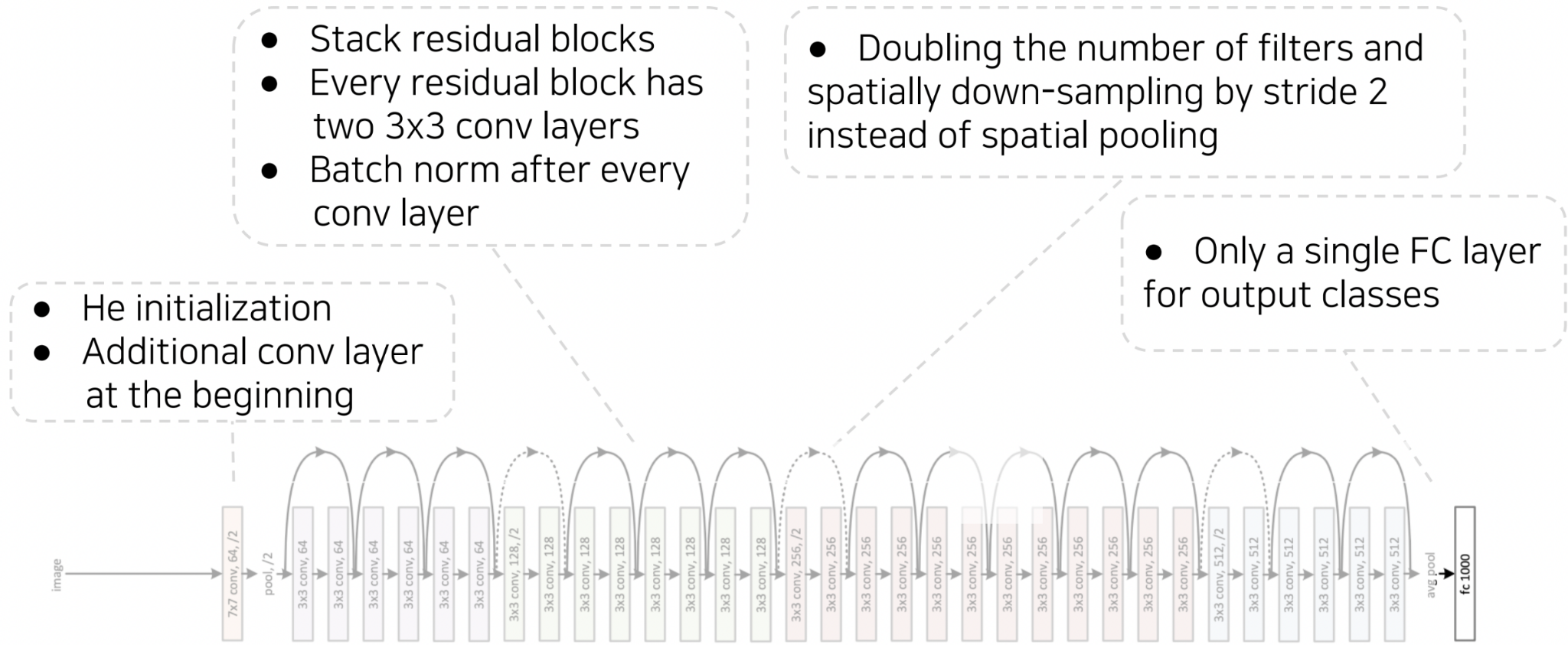
ResNet의 전체 구조는 7x7 convolution layer로 시작하여, residual block을 깊게 쌓아 구조를 형성한다. 각 block에서는 3x3 필터를 사용하며, block이 바뀔 때마다 공간 해상도는 절반으로 감소하고 channel 수는 두 배로 증가한다. 마지막으로 하나의 FC layer를 통해 최종 결과값을 출력한다.

PyTorch 기반 ResNet 구현
ResNet(18-layer)을 PyTorch로 구현한 코드를 살펴보면, conv layer → batch normalization → relu → max pooling을 통해 feature를 추출한 뒤, 이를 각 conv layer block을 거치도록 설계되어 있다.

각 conv layer block은 _make_layer 함수로 생성되며, 반복적으로 레이어를 중첩하는 구조이다. 마지막에는 average pooling을 통해 벡터화한 뒤, 하나의 FC layer를 통해 최종 logit 값을 출력한다. softmax를 추가하여 확률 값으로 변환할 수도 있다.

'MOOC' 카테고리의 다른 글
| [컴퓨터 비전의 모든 것] Semantic Segmentation (0) | 2024.12.20 |
|---|---|
| [컴퓨터 비전의 모든 것] Image Classification (3) : 모델 비교 (0) | 2024.12.20 |
| [컴퓨터 비전의 모든것] Annotation Efficient Learning (0) | 2024.12.20 |
| [컴퓨터 비전의 모든 것] Data Augmentation (2) | 2024.12.20 |
| [컴퓨터 비전의 모든 것]Image Classification (1) : 개념 (0) | 2024.12.20 |